My friend Corey, author of the excellent Bayesian Biologist blog, recently said:
“What I cannot create, I cannot understand” -Richard Feynman. This is why I always build a simulation of any problem I’m working on.
This post gives a good, elaborate example involving “trip taking behaviour of recreational boaters in Ontario.” I’ve recently been dabbling in statistical analysis but I’m not as much of a smartypants as Corey, so I’ve been using the same technique to learn basic statistical analysis.
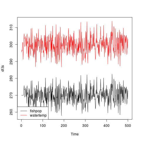
Here’s an example. When modeling time series (e.g., fish population and water temperature over time), it’s useful to detect if one variable has a dependence on the other at a certain log. Does a spike in water temperature at a given time cause an increase in fish a week later? The cross-correlation of water temperature and fish population would let us detect this relationship.
In R, there’s a handy ccf() function that will do this for me. But I’m not totally sure how it works, or what it looks like when it works. I’ll run it on some fake data to see what happens.
require(graphics)
# This is contrived, but let's pretend that water temperature is
# around 300 kelvin, +/- 5 kelvins. The error is normally distributed.
watertemp <- 300 + rnorm(500, 0, 5)
# This is even more contrived. Let's pretend that the fish population is
# around 270 in our pond, and that you can predict the population ten
# periods from now by multiplying the current water temperature by 0.9.
fishpop <- c(rep(270, 10), watertemp[11:500]*0.9)
x <- 1:500
df <- data.frame(fishpop, watertemp)
df.ts <- ts(df)
plot(df.ts, plot.type='single', col = 1:ncol(df.ts))
legend("bottomleft", colnames(df.ts), col=1:ncol(df), lty=1)
This is silly. But this lets me make a hypothesis about what the result of the ccf() function will be. I think it’ll show a correlation around 1 for a lag of 10. Let’s try it out.
ccf(fishpop, watertemp)
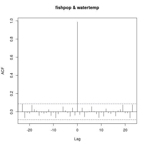
That wasn’t what I expected. This plot suggests that the two series are correlated without a lag. After a moment, I realize that there’s a bug in my code. The line
fishpop <- c(rep(270, 10), watertemp[11:500]*0.9)
does not produce a shifted time series; it just creates one identical to watertemp but with the first 10 values changed to 270. If I change this line to properly shift the series, I should see a correlation at lag = -10. Right?
fishpop <- c(rep(270, 10), watertemp[1:489]*0.9)
ccf(fishpop, watertemp)
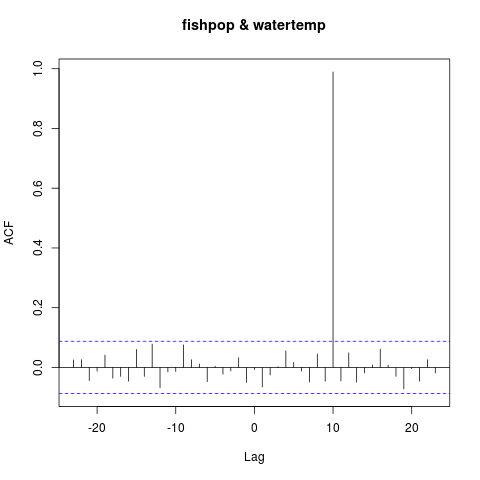
I was close. The correlation is at lag = 10. The correct way to read the plot is watertemp predicts fishpop ten periods later. Or, more simply, fishpop leads watertemp by 10 periods. Either way, I now have a better mental model of how the ccf() function works. If I applied it to real data, I’d be better equipped to interpret the results.
Most programmers do this instinctually in other domains. I certainly do. But with data analysis, my instinct is to run analyses on real data first — sometimes without really understanding what I’m doing.